To compute the consistency σ of all measurements, we assembled a network of half-cells. From these, cell I

Ag│AgZ_m (c, S₂) │ [N₂₂₂₅][NTf₂] │ AgZ_n (yc, S₁)│Ag                                   cell I

   ^{LJPS2                         LJPS1}

was built in 87 different combinations with the solvents S₁ and S₂ being water (H₂O), acetonitrile (AN), propylene carbonate (PC) and dimethylformamide (DMF). The latter were chosen as solvents, which dissolve silver salts AgZ readily and thus are expected to give stable potentials. In addition, part C of the liquid junction potential (LJP) was reported to be maximal for the water-DMF junction (> 100 mV according to Isutzu). It was therefore of interest to find out, if this contribution was relevant in our set up. The concentrations of the redox active salt AgZ used were set at 0.1, 1.0 and 10.0 mmol L⁻¹ and thus we expected the behavior of the dissolved ions to be almost ideal. As a control, we always implemented the MSA-model to approximate the activity coefficients of the half-cell electrolytes, and we found only small deviations (max. 2 mV) for the MSA corrected Δ_trG°(Ag⁺, S₁→S₂)-values.

Choice of Anions Z^– for AgZ: Six different anions Z⁻ were used as counterion for the silver cation (Figure). They stretch the range from rather small and stronger coordinating [NO₃]^–, [BF₄]^– to the medium sized triflate [OTf]^– (Tf = SO₂CF₃) and [SbF₆]^– (not shown), the larger triflimide [NTf₂]^– and the huge, almost ideally non-interacting [PF]^– (= [Al{OC(CF₃)₃}₄]^–).

The use of different counterions revealed only a minor influence on the cell potential. We deduce that the LJP is mainly determined by the IL constituting ions.

Network of Half-Cells: The next figure shows the assembled network. Mathematically, the network represents an overdetermined system, i.e. a system of equations with more equations than unknowns. The approximate solution can be found by the method of least squares. We use an established procedure, the result of which gives an optimized value for each unknown with an individual residue for each equation and an overall uncertainty expressed as σ.

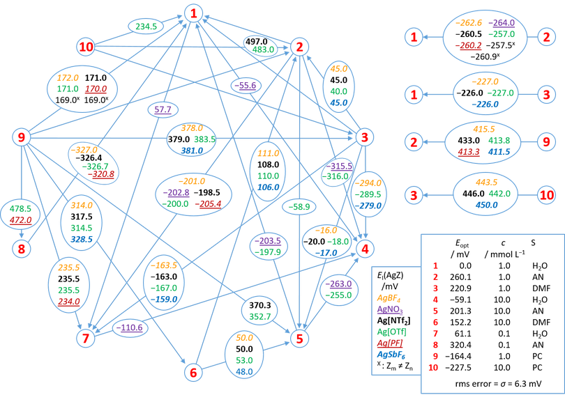
Caption to Figure Network Analysis: Sketch of the network of the half-cells, indicated by red digits 1…10, with the solvents S = H₂O, AN, PC and DMF in different AgZ-concentrations (c) in mmol L⁻¹ and with different anions Z⁻ (indicated by colors; Tf = SO₂CF₃, [PF] = [Al{OC(CF₃)₃}₄]). Each arrow between two points of the network symbolizes one distinct implementation of cell I. The starting point of the arrows is the right half-cell and the endpoint the left half-cell. The numbers in the circles superimposed on the arrows are the measured potential differences of cell I E_I in mV with the respective salts AgZ (encoded by colors). Some values are averages. E_opt is the optimized potential value with respect to half-cell 1 as the right half-cell obtained by the network analysis.

The results of our network analysis and additional literature data are summarized in Table 1. Δ_trG°(Ag⁺, S₁→S₂) values were obtained from the optimized half-cell values 1, 2, 3 and 9 according to the Figure above with both half cells having a concentration of 1 mmol L^–1. The quoted values obtained with different extra-thermodynamic assumptions (TATB, n-LJP and Fc) are discussed and compared to our results in a separate section below. The σ-value is essentially the root mean square deviation and was found to be 6.3 mV or 0.6 kJ/mol.

Table 1: Optimized values Δ_trG°(Ag⁺, S₁→S₂) from the network analysis. All energies in kJ mol⁻¹ (mol L⁻¹-scale). The range of individually measured values is given where available. Columns 4 – 6 refer to recommended values obtained with extra-thermodynamic assumptions.*

 * TATB: Δ_trG°(TA⁺) = Δ_trG°(TB⁻) for all S; n-LJP: neglection of LJPs; Fc: Δ_trG°(Fc) = Δ_trG°(Fc⁺) for all S. These are discussed below. ^a reference solvent AN; ^b reference solvent methanol; ^c calculated from the given column values (in case of ^b with additional values from Table V in the Ref.), i.e. not directly measurable (TATB- and Fc-method) or measured (n-LJP method).

Thus, the “ideal” ILSB-method delivers the currently most accurate experimental Gibbs energies of transfer of a single ion. In contrast to other methods, the consistency is high, shown by solid statistical analysis being 0.6 kJ mol⁻¹ resulting from the compilation of 87 measured values between four solvents. Being free from solvent-solvent interactions, the “ideal” ILSB provides considerable advantages against other methods, also due to the non-toxicity of the used IL in contrast to the picrates used by Alexander et al. Furthermore, with a suitable anionic redox system the thermodynamically rigorous determination of the LJP´s contribution of cell I is possible. Considering the small discrepancy to the quoted TATB-values being free of LJP-contributions (but certainly not of other, which may be summarized as asymmetric solvation of cation and anion) the x_I are small or – accepting the argument by Cox et al. as a simple approximation – even zero.

Current State: 145 measurements between a total of 12 electrochemical half-cells containing the six different solvents were executed forming a network expandable by additional redox systems as well as solvents. A statistical analysis on the complete current network disclosed a standard uncertainty of only ±5.7 mV or ±0.55 kJ mol^–1, which – compared to the (estimated) uncertainty of all other methods – is exceptionally good. The maximum deviation of all of the 145 measured values from the optimized network expectation value is below 1.6 kJ mol^–1.

Thus, we recommend the use of this “ideal” ILSB-setup to determine Gibbs energies of transfers of single ions.